Gaussian Process

What is a Gaussian Process?
A GP is simply a multivariate Gauss distribution. The idea is very simple; we have a multivariate Gauss distribution which includes both previous measurements(or train set) and targets(test set). Either previous measurement or target, I will call them dimensions. They are some dimensions in the Gaussian Process.

Since the multivariate Guassian Distribution has covariance between the dimensions, we generate a knowledge such that the measured values actually carry information for the targets. The only thing GP does is to predict the new points with this information.

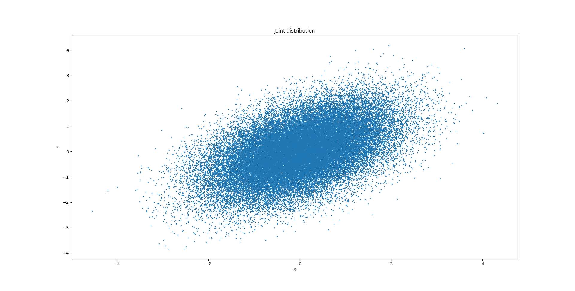
Consider the joint distribution with zero mean and with covariance matrix:

The joint distribution is:

Distribution of the single random variable P(X) is:

However, if we know the value of random variable Y, this means we will focus our search space for X into a new interval. This is because saying Y=1, for example, means we have an idea about X. Since Y and X are correlated, we have knowing Y=1 means X is also probably around these points. The distribution of X given Y is given by P(X|Y):

So, the idea is that. We have the measurement Y and now we can say something about X. Now think of it with many dimensions, but not only in 2 dimensions (X and Y dimensions). We can calculate the mean and covariance using the formula:

These two equations specify how our new kernel be when we predict a new point. The equations can be updated in an iterative manner. However, we can also calculate the conditional distribution, or our predictions, as:

TODO – maybe I can add some example here…

References:
[1] https://distill.pub/2019/visual-exploration-gaussian-processes/
[2] https://las.inf.ethz.ch/teaching/pai-f21

Code Snippet:

import matplotlib.pyplot as plt
import numpy as np
import pdb

BINS = 50
TRIALS = 50000

data = np.array([np.random.multivariate_normal([0, 0], np.array([[1, 1/2], [1/2, 1]])) for _ in range(TRIALS)])

plt.figure()
plt.scatter(data[:, 0], data[:, 1], 2)
plt.xlabel('X')
plt.ylabel('Y')
plt.title('Joint distribution')


#plt.show()

def inside_interval(arg, low, high):
    """Just return a boolean array inside the interval"""
    bool_array = np.zeros(arg.shape, dtype=bool) # all false

    bool_array[(arg > low) * (arg < high)] = True

    return bool_array

# assume we know first variable and want to find the second (we know Y)
one_dim = data[inside_interval(data[:, 1], low=0.9, high=1.1), 0]

plt.figure()
plt.hist(one_dim, bins=BINS)
plt.xlabel('X')
plt.ylabel('P(X|Y~=1)')
plt.title('Distribution of P(X) Knowing Y is around 1')


plt.figure()
plt.hist(data[:, 0], bins=BINS)
plt.ylabel('P(X)')
plt.xlabel('X')
plt.title('Distribution of P(X)')

plt.show()